**Solving the oxygen diffusion problem in Tomographic Volumetric Additive Manufacturing (TVAM) using inverse rendering**
Axel Stengel, student of [ENS Rennes](https://www.ens-rennes.fr/) and intern at the [RGL lab](https://rgl.epfl.ch/) under the supervision of Baptiste Nicolet and Wenzel Jakob.
Introduction
============
Tomographic Volumetric Addive Manufacturing or TVAM is an experimental additive manufacturing (AM) technology that allows very fast printing of models in resin.
The principle behing this technology is to use the transparent nature of the liquid resin in order to solidify the whole model at once unlike more classical methods like SLA ou DLP which print the model layer by layer.
This new approach encounters multiple physical effects that can alter the quality of the prints if not taken into account. In this internship we tackle the problem of oxygen diffusion in resin.
This internship is a continuation of the work of Baptiste Nicolet et al. [#Nicolet] in which they tackle other problems using inverse rendering such as non cylindrical vial, tilted rotation axis and scattering resin.
Background and related works
============================
TVAM
----
The theory behind TVAM relies on *computed tomography* (CT) [#Kelly] in which a patient or object is exposed to a rotating X-ray source.
The absorption of those rays is mesured with a sensor wich produces a set of patterns.
Those absorption patterns can then be used to reconstruct a 3d model of the target.
TVAM works the other way around, begining with a 3D model, we compute a set of patterns that we then expose to a rotating vial of *UV-sensitive resin* in order to create the physical model.
This means that over the duration of the print, some parts of the resin receive a higher dose of UV light leading to their polymerisation.
![Figure [TVAM]: The patterns are produced by a Digital Micromirror Device (DMD) that redirects UV light from a laser source onto the resin vial rotating at a constant speed. The DMD's surface is composed of tiny mirrors that can be oriented to only redirect a fraction of the incoming beam, allowing for more control on the exposure of the resin.](imgs/TVAM_figure.jpg width="300px")
Oxygen Diffusion
----------------
The *polymerisation process* of UV-sensitive resin is based on a chemical balance between an inhibitor (oxygen) and and a reagent (*free radicals*). On its own, there is much more oxygen disolved in the resing so any free radicals react with the oxygen to create inert byproducts or short chain polymers. However, when UV light of the correct wavelength is shone into the resin, previously inert molecules called *photo-initiators* are broken up and create free radicals. As those radicals react with the disolved oxygen, the oxygen concentration drops and once it is below a certain threshhold, not enough oxygen can react with the radicals and they begin forming *long chain polmers*, thus solidifing the resin.
![Figure [oxy_inhib]: The chemical reaction behind the polymerisation of UV-sensitive acrylate resin differs depending on the oxygen concentration in the resin, only producing long chain polymers when the oxygen concentration is low enough. [#Höfer] ](imgs/oxy_inhib.png)
In other resin printing techniques this polymerisation process only takes a few seconds as they only polymerise a thin layer of resin at a time. However, in TVAM, the time betwen first exposure and full polymerisation is much longer (usually 30 seconds to a couple of minutes) as we need to solidify the whole model at once. This means that over time, a gradient of oxygen concentration will form in the resin and oxygen from high concentration areas (outside the model) will diffuse into low concentration areas (inside the model) to try and level the gradient. This diffusion results in a blurring effect on the model, especially present on small details.
![Figure [oxy_diff]: The oxygen diffuses from high concentration areas (outside the model) into low concentration areas (inside the model).](imgs/oxy_diff_figure.jpg width="200px")
A previous approach to solve this problem considered the diffusion as a global convolution with a blurring filter. As such their approach consisted in deconvolving a simulated absorption grid and computing patterns based on it [#Orth]. While the results were promising, they ignored the time factor of the diffusion problem, as not all areas of the print volume are exposed at the same time and thus affected equaly by the diffusion.
Simulating absorption in resin
------------------------------
The patterns were originally computed using the *Radon transform* [#Kelly], a linear operator that takes a 2D slice of a model and returns a sinograph that represent the absorption along a set of angles. To compute the simulated absorption we can use the adjoint operator of the Radon transform called *backprojection*. This however produces a blurry result as many physical phenomenons are not taken into account, such as the fact that the absorption of the UV light is not uniform in the resin. An improved method known as *filterd backprojection* [#Bernal] can provide clearer simulated result but creates physically impossible negative regions which, if ignored, produce artifacts when printed.
![Figure [radon]: The combination of the Radon transform and its adjoint operator the backprojection produces a blurry result.](imgs/radon_trans.png width="300px")
A better approach to simulating absorption in resin is to use ray tracing with a physicaly acurate light transport model. These approaches can easily take into account non uniform light absorption, refraction on the glass vial or even scattering resin [#Nicolet]. This combined with a voxel grid [#Weisgraber] can produce physicaly acurate simulation of the absorption and polymerisation of the resin through accumulators that compute the absorption integrated over the print time. Our method uses two accumulators introduced by Nicolet et al., the ratio accumulator that samples points along the ray and the DDA accumulator that accumulate for every voxel traversed by the ray.
![Figure [Ratio]: The ratio accumulator samples point (blue) along the ray (red) and accumulates the chosen voxels (gray). This accumulator produces fast but noisy results.](imgs/ratio1.svg width="300px") ![Figure [DDA]: The DDA accumulator (digital differential analyzer) computes efficiently every voxels (gray) traversed by the ray (red) between an entry and exit point (blue). This accumulator produces slower but less noisy results.](imgs/DDA1.svg width="300px")
Inverse Rendering
-----------------
Our method is based on the use of inverse rendering to compute the patterns, an approach introduced by Nicolet et al..
Inverse rendering is a technique that combines a *differentiable forward rendering model* and a *gradient-based optimzer* to compute missing parameters in a scene based on a set of expected results. Inverse rendering can be used in a variety of inversion problems, from computing the colors in a scene to generating the geometry of an object.
![Figure [autodiff]: A scene with missing parameters is rendered with a differentiable model and the result is compared to the expected result with an objective function. This function is then fed into a gradient-based optimiser that updates the input parameters and interates until sufficient precision is obtained. [#Mitsuba] ](imgs/autodiff_figure.jpg)
Inverse rendering applied to oxygen diffusion
=============================================
Theory
------
Our approach is based on the theory that the oxygen diffusion can be better simulated by taking into account the fact that some part of the resin is exposed before others. As such, the absorption of the first patterns will be more affected by oxygen diffusion than others. Our solution uses the framework developed by Nicolet et al. where the DMD patterns are optimised from a start configuration through inverse rendering.
Rendering methods
-----------------
Our approaches to rendering the oxygen diffusion can be divided into two categories :
- the convolution methods serve as a ground truth for our forward renderer
- the sampling methods are much faster
### Convolution methods
The first convolution approach is the closest to the actual diffusion mechanism. We compute the absorption of the patterns seperately and convolve the aborption grid with a small gaussian kernel between each pattern. This small gaussian kernel represents the diffusion during the exposure time of one pattern and as such is of constant size.
~~~~~~~~~~~~~~~~~~~~~~~~~~~~~~~~~~~~~ python
absorption_grid = Tensor(res,res,res)
dt = print_time / nb_patterns
kernel = gaussian_kernel(sqrt(D*dt))
for i in range(nb_patterns) :
absorption_grid += render(patterns[i])
convolve(absorption_grid,kernel)
return absorption_grid
~~~~~~~~~~~~~~~~~~~~~~~~~~~~~~~~~~~~~
For the second convolution approach we shift our perspective from simulating small diffusion steps between patterns to simulating the diffusion a single pattern throughout the duration of the print. That means that the convolution is computed before adding the absorption to the voxel grid and that the kernel size decreases with time.
~~~~~~~~~~~~~~~~~~~~~~~~~~~~~~~~~~~~~ python
absorption_grid = Tensor(res,res,res)
dt = print_time / nb_patterns
for i in range(nb_patterns) :
kernel = gaussian_kernel(sqrt(D*(print_time - i*dt)))
temp = convolve(render(patterns[i]),kernel)
absorption_grid += temp
return absorption_grid
~~~~~~~~~~~~~~~~~~~~~~~~~~~~~~~~~~~~~
In theory, both methods should yield the same results as the convolution of multiple gaussians is a gaussian whose variance is the sum of the input gaussian's variances.
The issue with these methods is that we need to compute each pattern absorption seperatly, which is not optimal when rendering on GPU as it limits the parallelisation of the computation. One way to reduce the effect is to group patterns into small batches. That is, instead of computing the convolution between each pattern, we can render a small group of patterns at once and compute the diffusion during the timeframe of those patterns, thus having a smaller number of bigger computations.
### Sampling methods
Both our sampling methods rely on the same idea as the second convolution methods, the samples are coming from a gaussian with a kernel size decreasing with time. How exactly the voxels are sampled depends on the accumulator used.
For the ratio accumulator, we have exact points sampled along the rays, so we just offset each point by a gaussian sample. For the DDA accumulator however, we only know the begining and end point of the ray in the grid so we offset both of them by the same sample so that the whole ray is offset.
![Figure [Ratio2]: The modified ratio accumulator samples point (blue) along the ray (red) and offset them by a gaussian sample (green) before accumulating the chosen voxels (gray).](imgs/ratio2.svg width="300px") ![Figure [DDA2]: The modified DDA accumulator offset the whole ray (red) and computes every voxels (gray) traversed by the offsetted ray (green).](imgs/DDA2.svg width="300px")
Results & Discussion
====================
Implementation details
----------------------
The code is strongly based on the code of Nicolet et al., it is written in Python with the Mitsuba 3 render [#Mitsuba] and DrJit [#DrJit] JIT framework doing most of the computation and auto-differentiation and Torch [#Torch] used for the convolutions.
Rendering of the oxygen diffusion
---------------------------------
To test our rendering of oxygen diffusion, we rendered a benchy model [#Benchy] using pattern optimised without diffusion. The renders without diffusion produce a crisp result with a slightly noisier result for the ratio accumulator. For the convolution methods, we rendered them with batches of 10 patterns in order to limit the computation time as there was no visible difference between batches of size 10 and batches of size 1. The results are, as expected, a blurry rendering of the non-diffusion results where we see that small details are lost. The sampling methods produce a similar but noisier result.
  
  
![Figure [Rendering_table]: Rendering of the same slice with the different rendering methods. The rendering without diffusion, using the ratio accumulator (a) and the DDA accumulator (d) serve as the baseline. We can see that both convolution methods (c : first method, f : second method) produce the same result. The sampling methods also produce similar results to the convolution methods with the ratio accumulator (b) adding more noise than the DDA accumulator (e) as expected.](imgs/Empty.png)
To better understand the time dependent effect of the oxygen diffusion, we can look at a small slice of the model. Here we clearly observe that the diffusion is more severe ar the top of the slice as it is the first exposed portion of the resin.
![Figure [Showcase]: The render with diffusion simulation (left) compared the render without diffusion (left) shows that the blur is not uniform and parts that are exposed first show more diffusion.](imgs/Empty.png)
All four methods are theoreticaly differentiable, however the convolution methods require too much memory to keep track of the AD graph as in the current implementation each convolution gradient result need to be kept in memory. This can easily consume more VRAM than even an high-end GPU like the RTX 4090 can provide (24Gb).
Optimisation of patterns
------------------------
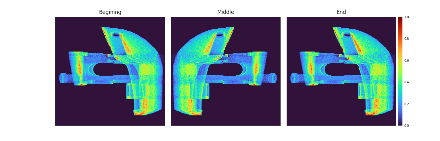
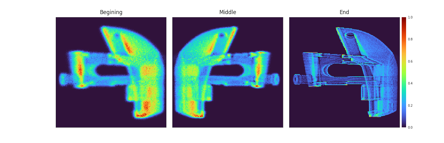
The following figures compare the patterns optimised with and without diffusion during the optimisation. The other parameters remain the same for both optimisation.
When looking directly at the pattern, we notice that, while the distribution of intensity in the patterns optimised without diffusion is mostly constant throughout the patterns, when optimised with diffusion, the first patterns are much more intense than the last. The first patterns are also blurier that the last that are sharp. This indicate that it is optimal to expose the bulk of the model first and render the finer details later in order to try and keep their sharpness.
![Figure [Benchy_patterns]: Optimised patterns with (left) and without (right) diffusion. When optimised with diffusion, most of the exposition happens in the first half of the patterns with a blurry approximation of the object. The finer details are exposed in the later half in order to reduce the effect of diffusion on them.](imgs/Empty.png)
The result of this are very promising as the simulated print shows much better detail retaintion than with non-diffusion optimised patterns. Notably the sidewalls of the benchy keep their thickness and angles much better then without diffusion.
![Figure [Benchy]: Rendering and approximation of the final result with patterns optimised with (left) and without (right) diffusion. When diffusion is not taken into account, the simulated result loses a lot of the finer details like the side walls of the benchy. When the patterns are optimised with diffusion, those details are mostly kept and the result is much closer to the target.](imgs/Empty.png)
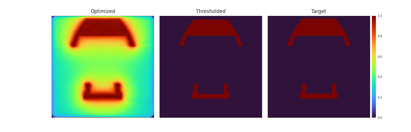
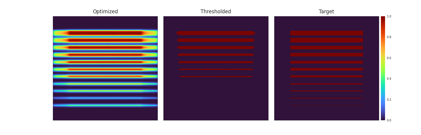
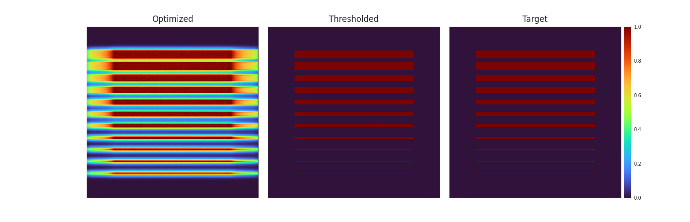
On a more pathological model, the result are even more impressive. The diffusion disks introduced by Orth et al. showcase exactly the problem of oxygen diffusion. In the simulated print with non-diffusion optimised patterns, the thinner disks completely disapear and there is a considerable ammount of bleeding at the edges of the bigger disks. The patterns optimised with diffusion however produce an almost perfect result with all disks present and mostly clean edges.
![Figure [Disks]: Rendering and approximation of the final result with patterns optimised with (left) and without (right) diffusion. The disks showcase exactly the problem of oxygen diffusion, without factoring in the diffusion when optimising the patterns, the thinner half of the disk is missing and there is a considerable ammount of bleeding at the edges of the bigger disks. The patterns optimised with diffusion produce an almost perfect result.](imgs/Empty.png)
Discussion and future works
---------------------------
The results of the optimised patterns using our forward model are very promising and show considerable improvement in simulated print quality. However, in this internship, we did not have time to actually print a test model with these patterns.
Another possible improvement would be a better implementation of the convolution methods in order to reduce their memory consumption and make them usable in optimisation.
Bibliography
============
[#Nicolet]: Baptiste Nicolet, Felix Wechsler, Jorge Madrid-Wolff, Christophe Moser, and Wenzel Jakob. 2024. Inverse Rendering for Tomographic Volumetric Additive Manufacturing. *In Transactions on Graphics (Proceedings of SIGGRAPH Asia)* 43(6). 1-17, 2024. https://doi.org/10.1145/3687924
[#Kelly]: Brett E. Kelly, Indrasen Bhattacharya, Hossein Heidari1, Maxim Shusteff, Christopher M. Spadaccini, Hayden K. Taylor, Volumetric additive manufacturing via tomographic reconstruction. *Science* 363, 1075-1079, 2019. https://doi.org/10.1126/science.aau7114
[#Höfer]: Michael Höfer, Norbert Mozner, Robert Liska, Oxygen scavengers and sensitizers for reduced oxygen inhibition in radical photopolymerization. *J Polym Sci Part A: Polym Chem* 46: 6916–6927, 2008. https://doi.org/10.1002/pola.23001
[#Bernal]: P. N. Bernal, P. Delrot, D. Loterie, Y. Li, J. Malda, C. Moser, R. Levato, Volumetric Bioprinting of Complex Living-Tissue Constructs within Seconds, *Adv. Mater.* 2019, 31, 1904209. https://doi.org/10.1002/adma.201904209
[#Weisgraber]: T. H. Weisgraber, M. P. de Beer, S. Huang, J. J. Karnes, C. C. Cook, M. Shusteff, Virtual Volumetric Additive Manufacturing (VirtualVAM). *Adv. Mater. Technol.* 2023, 8, 2301054. https://doi.org/10.1002/admt.202301054
[#Orth]: Orth, A., Webber, D., Zhang, Y. et al. Deconvolution volumetric additive manufacturing. *Nat Commun* 14, 4412 (2023). https://doi.org/10.1038/s41467-023-39886-4
[#Mitsuba]: https://mitsuba.readthedocs.io/en/stable/index.html
[#DrJit]: https://drjit.readthedocs.io/en/stable/
[#Torch]: https://pytorch.org/docs/stable/torch.html
[#Benchy]: https://www.3dbenchy.com/